extracted with some modififications from B. Frick, 'Neutron Backscattering' in HERCULES LECTURE NOTES, 2005
‘ Fixed window scans ’ or ‘ elastic scans ’ are very popular on BS spectrometers, but can also be employed on any neutron spectrometer which does not use the time-of-flight method. Fixed window scans are powerful for getting a fast overview over the dynamics of a system and are often the starting point for inelastic neutron investigations. How is it done?

 

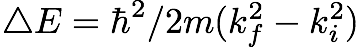
The monochromator and the analysers are chosen to reflect neutrons with fixed wave vectors k i and k f (i.e. they are not moving with time t and the lattice spacing does not change with temperature T). Thus, because k i (t,T)=const and k f (t,T)=const we analyse scattered neutrons within a fixed energy window . Now we can scan a sample parameter ( l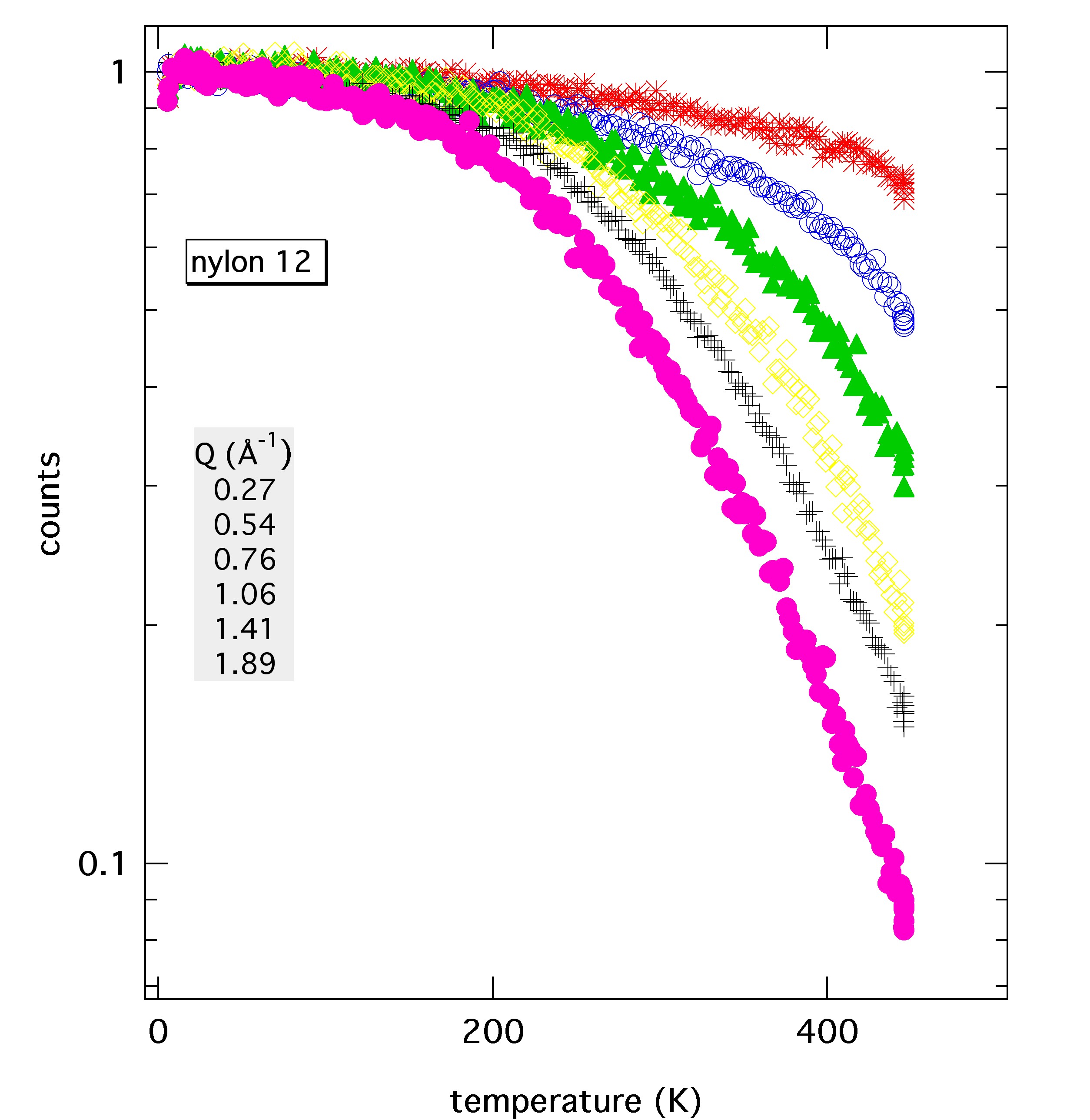ike temperature, pressure …) which then might influence the dynamics of the sample. For k i =k f we have the most commonly used ‘ elastic scans ’ for which ΔE=0 (this is the case if the monochromator is at rest and has the same crystals, orientation and temperature as the analysers). For k i ≠k f we deal with inelastic ‘fixed window’ scans 1 .

 

We can associate a frequency or time scale with the fixed energy window: e.g. if ΔE=0 and the instrumental resolution has a typical value for cold neutron reactor BS instruments of HWHM~0.4μeV, then this corresponds to a frequency of ν R ~10 8 Hz=0.1GHz, thus to a time window of observation of about 10ns or 0.01μs (using the conversion 1THz=4.136meV). Dynamic processes on a time scale slower than the instrumental resolution are not resolved and thus are counted within the ‘elastic window’. Faster motions of scattering particles can be resolved and will induce an energy loss or gain of the scattered neutrons (k i ≠k f ), which then are no longer reflected by the analysers to the detectors. In that case one observes a decrease of the elastic window intensity as function of the recorded variation parameter.

 

 If we analyse for k i ≠k f , (e.g. monochromator and analyser are at a different temperature, or have a different orientation), then one can find an increase of intensity in the fixed observation window or even a maximum as function of the variation parameter, when e.g. the dominating relaxation frequency of a dynamic process corresponds to the ‘fixed window’ frequency ΔE±HWHM (earliest example for such a scan 1 ).

 

The fixed window method has the advantage that the total counting time is spent in one channel, which corresponds to a large intensity gain. Elastic scans can be simulated assuming a model scattering law for e.g. the temperature dependence. Such an evaluation should be done with some caution and one should keep in mind that direct spectroscopic information is lost and the number of free fit parameters is usually larger than for spectroscopy. Therefore it is in any case advisable to complete the scans by inelastic spectra at several parameter points.

 

The parameter dependence of the scattering can give information e.g. on the activation energy of a dynamic process. Furthermore the spatial spatial information is deduced form the angular or Q-dependence (Q el =4π sin(Θ/λ) of the scattering.

 

For incoherent scattering the integral over the dynamic scattering law must be one: . If the measurement is carried out at very low temperatures, then we can consider the dynamics to be so slow that a BS instrument is not able to resolve it. Furthermore the Q-dependence will be flat (no motion) if we assume that the Debye-Waller factor is unity (we neglect zero-point motion). Thus an elastic window experiment at low temperatures can be used for normalisation onto the total scattering, after subtraction of background. This also removes other correction factors, which usually are more difficult to handle. It does not treat correctly multiple scat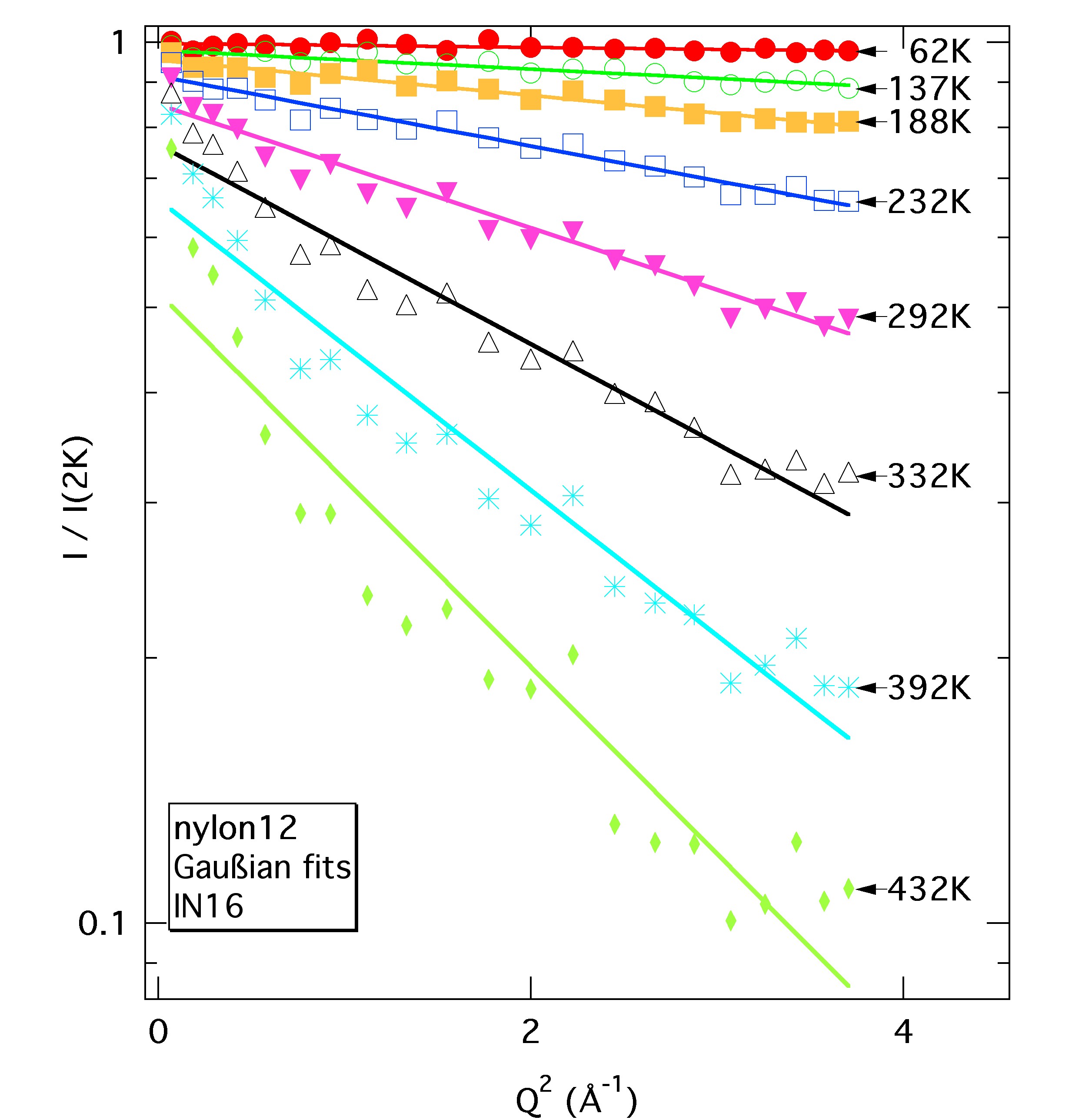tering effects, however, and artefacts may be produced if the sample scattering is coherent and changes with the scan parameter. For dominantly incoherent scattering and quasielastic processes which are fast on the time scale of the BS-resolution, the elastic intensity is a good measure of the Elastic Incoherent Structure Factor (EISF).

 

An example for such a fixed window scan is on this page, The first figure shows the measured elastic intensity as a function of temperature for nylon-12, a polymer with long methylene sequences. With temperature the motion of these –(CH 2 )- units becomes increasingly faster (e.g. vibrations, librations, trans-gauche transitions etc.) and thus leads to a loss of elastic intensity. As explained above, the data are normalised to the lowest temperature. From the Q-depend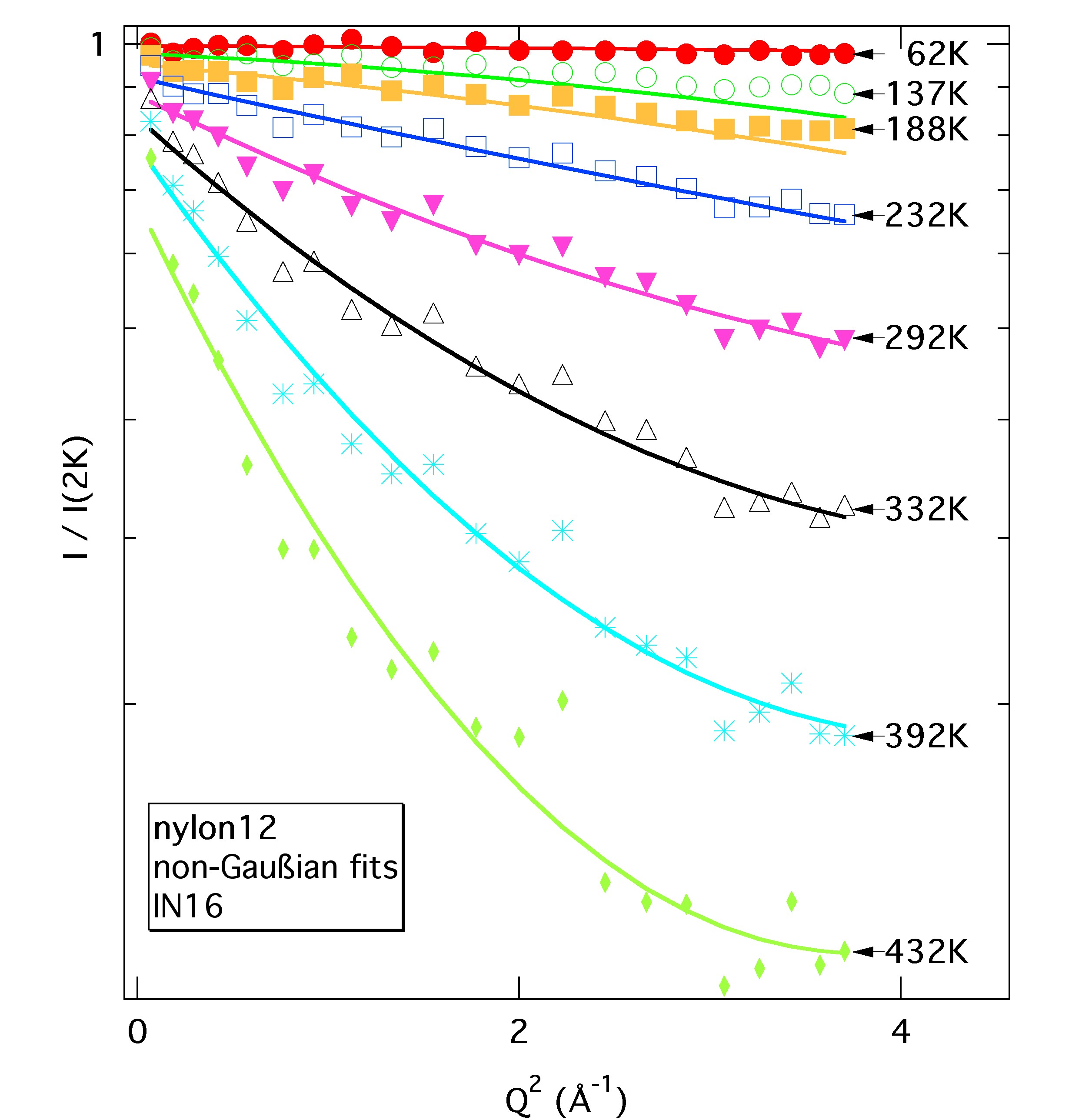ence one can deduce information on the spatial extend of the motion and from the T-behavior in simple cases information on the activation energies. Model fits have to be carried out then for the temperature and Q-dependence, as shown here for two simple cases. In the second figure a fit with a harmonic vibrational model is attempted (I=I 0 exp(-1/3Q 2 <u 2 >); linear fits of ln(I) versus Q 2 , plus an additional constant contribution y frac , which may be partially due to multiple scattering events). In the 3rd figure an addition exponential term ~Q 4 is added (non-Gaussian model). 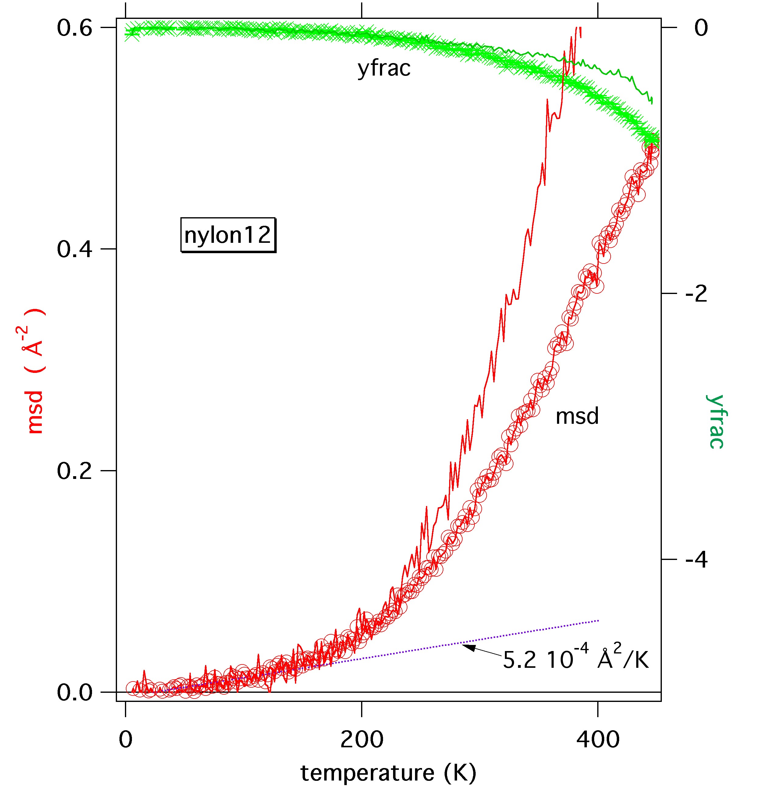An important resulting fit parameter is the T-dependence of the average mean squared displacement (of all protons in the sample), which is shown in the last figure (red), together with the constant y frac -term (green). The non-Gaussian term is not shown. As can be seen a harmonic vibrational model is only valid at low temperatures (roughly linear increase of <u 2 > with T). Above about 200K a different model has to be used. This can be a form factor for a specific molecular motion involving also an activation energy term or a more simplified non-Gaussian fit as done here. In our case the latter describes the data somewhat better.

 

1     H.-H. Grapengeter, B. Alefeld, and R. Kosfeld, Colloid & Polymer Sci. 265 , 226 (1987).