D17
Neutron reflectometer with horizontal scattering geometry
COSMOS is a program that will take raw TOF data for multiple angles, it will calibrate to the incident wavelength distribution and the detector efficiency, and will output reflectivity vs. Q. An article about the mathematical body of the program can be found here ("Towards generalized data reduction on a chopper-based time-of-flight neutron reflectometer", P. Gutfreund, T. Saerbeck, M.A. Gonzalez, E. Pellegrini, M. Laver, C. Dewhurst, R. Cubitt. Journal of Applied Crystallography 51, 606-615 (2018).).
Start the program by typing COSMOS in the LAMP manipulations window.

Note that, due to width specifications, a column is usually hidden to the right of the window. Use the slider bar at the bottom of the COSMOS window to find it.
Load/Save
This field allows you to save the current COSMOS configuration, or to load one that you have saved previously.
The configuration, with the name you give here, will be saved in the directory that you have specified in the IO path.
Data Table
The Data Table is a spreadsheet-like interface that allows you to enter the relevant file names and to force certain calculation constraints on COSMOS.
Each row corresponds to a separate reflectivity calculation.
The Direct columns are for the main beam measurements.
You can put multiple file numbers in here,
separate consecutive files by ',' (e.g. 12345,12347 will load 12345, 12346 and 12347)
separate non-consecutive files by a '+'. (e.g. 12345+12347 will load 12345 and 12347)
The Reflect columns are for the file numbers referring to the reflected beams. The post scripts '1' and '2' must correspond to the appropriate Direct post scripts.
You can put multiple file numbers in here,
separate consecutive files by ',' (e.g. 12345,12347 will load 12345, 12346 and 12347)
separate non-consecutive files by a '+'. (e.g. 12345+12347 will load 12345 and 12347)
The Normalise column can contain a constant, which will be used to multiply the calculated reflectivity.
This is useful if the sample is over-illuminated, in which case the reflectivity below the critical edge will be less than unity.
The Factor column can contain a constant, which is a relative scale factor between the first and second angles.
Because the oscillating slit is often used to measure the main beam at the second angle position, the calculated second angle reflectivity will be larger than reality. COSMOS will calculate a scale factor based on the reflectivities that overlap between the first and the second angles, however you can use this column to force the scale factor if you wish.
The Theta columns allow you to force the incident angles for the calculations of Q for the reflectivity.
You can enter a number here, or you can insert 'san' (where COSMOS takes the sample angle value from the data file), or 'dan' (where COSMOS calculates the value of theta based on the position of the reflected beam on the detector).
Probably the best thing to insert here is 'dan'.
The Out File column allows you to specify a name for the output data.
If nothing is chosen, the output will be saved under a name using the first run number in column 'Reflect 1'.
The Out LAMP column allows you to choose a LAMP workspace to output and view the calculated reflectivity.
Increment column(s): An easy way to enter data in to the table. Left click and drag in the cells of a column that you want to fill, enter the increment in the box, and click the 'Do' button. Hey presto! Filled columns!
This is particularly useful for entering the Direct Beam measurements. Use an increment of zero in this case.
Third angle: If a third angle is measured during the experiment, this option will create new columns in the data table.
Instrument Backgrounds: If you have measured the background in a separate measurement, choosing this option will insert up to three columns to allow you to enter the appropriate file numbers.
- These are the columns for the background file numbers for angles 1, 2 and 3 respectively.
IO
Data path:
Enter the path to your data and the path to output files here. If you're trying to access data while at the ILL, here's a couple of useful paths:
While using LAMP on the D17 instrument: /users/data/
If trying to access data from the D17 PC: \\serdon\illdata\yyc\d17\exp_x-xx-xxx\rawdata\
(yy = year, c = cycle. e.g. second cycle, 2005, = 052)
(exp_x-xx-xxx is your experimental number e.g. exp_9-11-1234)
Don't forget the last slash!
Output directory:
This is the directory where COSMOS will save the reduced ascii files and the cosmos setting files.
We recommend to use the 'processed' folder related to your experiment: \\serdon\illdata\yyc\d17\exp_x-xx-xxx\processed\
(yy = year, c = cycle. e.g. second cycle, 2005, = 052)
(exp_x-xx-xxx is your experimental number e.g. exp_9-11-1234)
Don't forget the last slash!
Output basename:
This is the name for the settings file.
Output file format:
Click here the data output formats you want to be saved.
MFT file contents:
This is the instrument parameters you want to be saved in the file header of the .mft file format.
Calculation
The calculation options tab controls the parameters used for finding and integrating the specular peak intensity, specifying the available wavelength range, subtracting background, and rebinning the data.
Clicking this tab will show something like the image on the right.
You have the possibility to enter different parameters for each of the measured angles.
Information on the individual fields is given below.
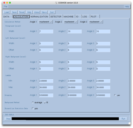
Calculation method: Here you can choose to add foreground intensities along lines of constant wavelength, which is the right choice if the sample is flat and the incoming beam divergence is higher than the detector resolution (incoherent method), or you can choose to add foreground intensities along lines of constant qz, which is the right choice if the sample is bent or the detector resolution is higher than the incoming beam divergence. In any case COSMOS will warn you in hte log tab if you have choosen an inapropriate method. Details can be found in: Cubitt et al., J. Appl. Cryst. 48, 2006-2011 (2015).
Foreground Width: COSMOS will look for the specular ridge, and will integrate the intensity over the number of x-pixels given by the number in this box. For example, if the number is 13, COSMOS will find the pixel corresponding to the centre of the specular ridge at x-pixel N and will integrate the intensity in x-pixels N — 6 < x < N + 6. You can also choose an asymmetric foreground width by typing in two numbers separated by a comma: e.g., if the numbers are 6,5, COSMOS will integrate the intensity in x-pixels N — 6 < x < N + 5.
Background Range: The range of x-pixels used to calculate the background is calculated from the limits of the foreground width. A single number will estimate the background from the pixels immediately from the limits of the foreground width. Two numbers, separated by a comma, estimate the background over a range of pixels given by the first number, spaced from the limit of the foreground by the second number.
For example, a specular peak centred at pixel N and a foreground width of 13 will have a left limit of N – 6.
A left range of 5 will use pixels N – 11 < x < N – 7 to estimate the background.
A left range of 5,5 will use pixels N – 16 < x < N – 12 to estimate the background.
Lambda Range: The wavelength range, calculated from the time-of-flight and from the incident angle of the beam, that will be used for the reflectivity. A wavelength range of 2 to 20 Å is normally reasonable.
Background Method: The two options to choose between are:
Average – This will simply take the mean of the intensity in the background range, and subtracts this mean from each point under the specular peak. This should be fine if the background is roughly flat over the pixel range, and the peak shape of the specular scattering, projected on to the x-pixel axis, is symmetric.
Fit – This assumes that the background is linear around the range of the peak. A straight line is fitted through the background points, and the background contribution for each point under the reflection is calculated based on the resulting equation. This may give better results if the peak shape of the specular scattering, projected on to the x-pixel axis, is not very symmetric.
Grouping: This will rebin the data, producing a smoother plot.
If 'Grouping' is selected, COSMOS applies a grouping based on the calculated resolution of D17, δQ. This resolution changes as a function of Q. The value entered is multiplied by δQ(Q) and, after grouping, will give the new distance between one point and its neighbour.
e.g.:
The raw data for a particular measurement:
Q1 = 0.0100003, δQ1 = 0.000264723
Q2 = 0.0100197
Q2 – Q1 = 0.0000194
(estimates come from unbinned data. δQ is the estimated FWHM of the resolution)
Assume that a Parameter value of 0.2 is chosen.
The step size between Q1 and the rebinned neighbour, Q2’, wil be 0.2× δQ1.
i.e. Q2’ – Q1 = 0.2 × 0.000264723 = 0.0000529446
The data within this interval will be averaged to a single point.
Discard Low Statistics Data: This runs a routine that cleans up noisy data.
After the data at all angles have been combined and sorted by ascending Q, the routine searches through neighbouring pairs of data. The criteria for considering rejection is when the q-resolution range for Q on one of the data points fits entirely within the q-resolution range for the other.
e.g. consider two points:
Q1 = 0.010, δQ1 = 10–4
Q2 = 0.011, δQ2 = 0.005
The tolerance range for Q1 (0.0099 ‹ Q1 ‹ 0.0101) is within the tolerance range for Q2 (0.006 ‹ Q1 ‹ 0.017). This satisfies the criteria for rejection.
The routine then rejects the data point with the largest error on the reflectivity. NOTE: Using this routine you effectively discard information. We therefore do not recommend to use this option for data to be fitted. This option is reserved for cosmetics in Figures only.
The 'Normalization' tab
This tab gives you the possibility to access the following settings/calulcations:
Normalization: Here you can calculate the normalization and attenuation factors from a direct beam measurement (called 'Direct beam') and reflected beam measurments (called 'D2O'), where the first angle should have some total reflection in the q-range defined 'Q range'. Entering the respective numbers ain the fields, optionally providing the refelction angle and clicking on 'Calculate' will make the corresponing factors appear. You can transfer them to the Data table by clicking 'Transfer factors' button. You can do the same transfer with the direct beam numbers and the Sample theta values.
Beam normalization: Here you can choose between normalizing to the monitor counts or the counting time.
Detector calibration: Here you can provide a water run number to correct for detector efficiency.
Polarization correction factors: Here you should provide a file name for the instrument polarization inefficiencies, which should be provided by your local contact in case you used polarization/analysis.
Detector
Clicking this tab will open a window that allows you to select the areas of the detector where COSMOS will search for the specular reflection. This is a useful option if there is strong, structured off-specular scattering, or for weak reflectivity.
Pixel range: Specify here the first and last x-pixels in the detector range to be used, separated by a comma.
The D17 detector has 256 pixels in the x-direction. Look closely, and you will see that the first and last 20 or so pixels have zero intensity. In other words, the x-range is larger than the range on the detector. For this reason, it is best to always have an x-range of something like 30 ≥ x ≥ 245.
Search Range for Peak: Specify the ranges (x detector pixels) of the detector that will be used to find the specular reflectivity.
Search Range for Peak (TOF channels): The minimum and maximum y-detecor pixels that will be used to find the specular reflectivity.
In time-of-flight, the specular reflectivity corresponds to a vertical line on the detector. COSMOS will look for a peak within the range that is defined in x integrating over the range defined in y (TOF channels).
Leaving the fields blank means that no limits will be adopted.
Inserting auto in the TOF channels field means that the reflectivity will be calculated over the wavelength range defined in the Calculation tab.
Machine
The Machine tab contains very important parameters that come from the calibration of time-of-flight parameters on D17. Make sure that they are correct with respect to your measurement!
You can ask your local contact for the correct parameters.
Usually, the correct values should be saved in the data file. In this case you just untick the 'Override numors values' box.
d0,d1: This is the distance between the choppers and the sample position, given in metres.
Opening Offset: If the choppers are phased to this value, the beam has no direct line of sight from the guide to the sample position.
Poff Offset: This is a parameter giving twice the angle between a pickup on the chopper (from which the time-of-flight is calculated) and the opening edge of the chopper.
TOF delay: This is the electronic delay time between the pick-up pulse of the master chopper and the start of the detector acquisition in seconds.
Sample position offset: This is an offset of the sample position from the center of the goniometer stage on FIGARO. Positive direction is away from the reactor, so typically this should be a negative number if the sample is placed closer to the sample slit. This is usefull to minimize the gravity effect. Note: This option is not implemented for D17!
Pixel Width: This is the width of an x-pixel, given in metres.
Sample-to-detector distance: This is the distance from the sample centre to the detector in metres. In case of FIGARO this is the distance for the direct beam configuration.
Distances: These are the distances of the detector translation stages on FIGARO from which COSMOS calculates the actual sample-to-detector distance for any configuration. This is needed as the FIGARO detector is not rotating around the sample, but can be placed in any position.
Take values from numor: Here one can type in an experimental file number and COSMOS will read the machine parameters from this file when clicking on 'Take'.
Override numor values: The above values should be saved in the data file, and they should be read automatically when COSMOS is run. If you suspect that the values are wrong, you may click this option and manually enter the values.
You have the possibility to have different values for each angle measured.
On D17 these values are usually the same for all angles. They will sometimes change between cycles if there has been an intervention on the instrument. The only time you would need to have different values for different angles would be if you wanted to analyse sets of data from the same sample, measured in separate experiments (this is generally inadvisable anyway).
On FIGARO these values will change between angles. Make sure you keep a record of the right values.
Ask your local contact and/or the instrument responsible for more details.
Data overlap regions
The useable wavelength range on D17 is typically 2.2 – 27 Å. This means that D17 can simultaneously cover an order of magnitude in Q.
This is generally not enough to cover a full reflectivity curve, however. Hence, measurements must be made at at least two angles. There will be some overlap of data between these angles.
This page describes what COSMOS does automatically if the 'Factor' column is kept empty. Alternatively the same factor can be calculated in the 'Normalization' tab and transfered to the whole table by clicking on the 'Tranfer' button. It is also possible to type in the attenuation factors by hand if they are known or derived from matching the respecive parts of the reflectivity manually.
Step 1: Calculation of the 'reflectivity' for the separate angles
The 'reflectivity' of the separate angles is calculated. This calculation finds the specular reflection (within the defined search range of the detector), subtracts background, corrects for detector efficiency (water), and divides the reflected data by the direct beam.
Normally, this gives the reflectivity. However, particularly for the direct beam at larger angles, the oscillating attenuator is often used to avoid detector saturation. For this reason, there may be a (constant) multiplicative factor which must be accounted for.
Step 2: Determination of the overlap region
The Q values for the different angles are calculated (acoording to the wavelength ranges given in the 'Calculation' tab) and the overlap region between angular data sets is determined.
Step 3: Interpolation of Q
Within the overlap region, the Q-values for the larger angle are interpolated on to the Q-values for the smaller angle. There will then be N points spanning the overlap region, where N is the number of Q-values for the smaller angle within the overlap region.
Step 4: Determination of the scaling factor
The ratio is calculated for the data at each of the matching Q (actual Q for the smaller angle, interpolated Q for the larger angle).
The ratios are then weighted by the reciprocal of the statistical error in each point.
The scaling factor between the higher and the lower angles is then the mean of the weighted ratios.
Step 5: Scaling of the larger angle
All of the higher angle data is then multiplied by this factor.
Step 6: Grouping
The individual angles are then rebinned using the Group Data function (if requested).
Step 7: Returning the result
The combined data set is then returned to COSMOS and saved.
Data Output Formats
COSMOS will output up to five output files for each of the reflectivity profile that it calculates, depending on the formats chosen in the IO tab. The output files are all in ASCII.
The names of the files are identical, with different extensions. You may choose the names of the files using the Out file column in the Data Table. If this is not defined, the names of the files will be the number of the first run at the first angle.
The five types of file are:
*.out
This is an ASCII file that contains relevant information about the calculation and returns the unbinned and unscaled data, along with the estimates for the q-resolution (FWHM) at each point.
The file has 22 lines of header information before the data begins. The header summarizes the run numbers and calculation conditions for COSMOS.
The 22nd line has the labels for the data columns.
The data are in 4 columns, which are (in order): scattering vector (in Å–1); reflectivity; error; resolution (FWHM) (in Å–1).
The format of each row is:
<number> <blank> < number> <blank> < number> <blank> <number>
where each number occupies 13 characters.
The number of rows in the data depend on the number of time-of-flight channels used and the calculation parameters using in COSMOS.
You can find an example of a *.out file here.
*.dat
This is an ASCII file with 3 columns of data and no header. The columns contain (from left to right) the values of Q (in Å–1), reflectivity and the error respectively.
This data file may be directly loaded in to the PARRATT32 reflectivity program. Note that negative reflectivities are omitted.
You can find an example of a *.dat file here.
*.aft
This is an ASCII file with a four line header and 3 columns of data. The columns contain (from left to right) the values of Q (in Å–1), reflectivity and the error respectively.
This data file may be directly loaded in to the AFIT reflectivity program.
You can find an example of a *.aft file here.
*.mft
This is an ASCII file with some metadata in the file header depending on the parameters chosen in the IO tab and 4 columns of data. The columns contain (from left to right) the values of Q (in Å–1), reflectivity, error and resolution (FWHM in Å–1), respectively. The data is binned and normalized.
This data file may be directly loaded in to the Motofit reflectivity program.
*.lam
This is an ASCII file identical to the *.mft format but with a fith columns of data corresponding to the wavelength in Å. This is important if the reflectivity becomes wavelength dependend, as is the case for very thick layers (more than 1 micron) or nuclei with resonances in the chosen wavelength range (e.g. Gd).